• Table of Contents

  • Comparing Two Columns in Excel: A Comprehensive Guide
  • Method 1: Using Conditional Formatting
  • Method 2: Using Formulas
  • Method 3: Using VLOOKUP
  • Conclusion

Comparing Two Columns in Excel: A Comprehensive Guide

Excel is a powerful tool that allows users to manipulate and analyze data in various ways. One common task that users often need to perform is comparing two columns of data to identify similarities, differences, or patterns. In this article, we will explore different methods and techniques for comparing two columns in Excel.

Method 1: Using Conditional Formatting

Conditional formatting is a handy feature in Excel that allows users to apply formatting rules based on specific conditions. This can be useful for visually highlighting differences between two columns. Here’s how you can use conditional formatting to compare two columns:

• Select the two columns you want to compare.
• Go to the “Home” tab and click on “Conditional Formatting.”
• Choose “Highlight Cells Rules” and then “Duplicate Values.”
• Select the formatting options you prefer, such as highlighting duplicate values or unique values.

By using conditional formatting, you can quickly identify duplicate or unique values in the two columns, making it easier to spot any discrepancies.

Method 2: Using Formulas

Another way to compare two columns in Excel is by using formulas.

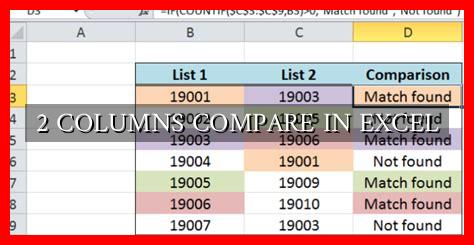
. One common formula for this purpose is the =IF function. Here’s how you can use the =IF function to compare two columns:

• Create a new column next to the two columns you want to compare.
• Enter the formula =IF(A1=B1, "Match", "No Match") in the first cell of the new column.
• Drag the fill handle down to apply the formula to all rows.

This formula will compare the values in cells A1 and B1 and return “Match” if they are the same, or “No Match” if they are different. You can then filter or sort the new column to easily identify matching or non-matching values.

Method 3: Using VLOOKUP

VLOOKUP is another powerful function in Excel that can be used to compare two columns and retrieve corresponding values. Here’s how you can use VLOOKUP to compare two columns:

• Create a new column next to the two columns you want to compare.
• Enter the formula =VLOOKUP(A1, B:B, 1, FALSE) in the first cell of the new column.
• Drag the fill handle down to apply the formula to all rows.

This formula will search for the value in cell A1 in column B and return the corresponding value. If a match is found, it will display the value; otherwise, it will return an error. This can be useful for identifying common values between the two columns.

Conclusion

Comparing two columns in Excel is a common task that can be accomplished using various methods and techniques. Whether you prefer using conditional formatting, formulas, or functions like VLOOKUP, Excel offers a range of tools to help you compare and analyze data effectively. By utilizing these methods, you can gain valuable insights and make informed decisions based on your data.

For more advanced techniques and tips on data analysis in Excel, check out this Excel tutorial website.